How a model got its weights

The science of LLM training dynamics.

While writing this piece, an excellent position paper came out on arXiv (Biderman et al., 2026), articulating some of these same arguments about the importance of analyzing training dynamics. I’ve tried to weave some of those arguments into the current piece, but I also highly recommend that interested readers check out the paper!

---

A large language model (LLM) does not appear out of nowhere. It is the result of subjecting a neural network—typically with a random initial configuration of weights—to an extensive training process. During this training process, an LLM’s weights are updated in ways that, hopefully, improve its ability to predict tokens in the kinds of contexts it’s been exposed to.

Much of the enthusiasm around LLMs comes from the observation that this simple training procedure results in systems that produce, for lack of a better term, interesting behaviors. There’s considerable debate about how to measure these behaviors and whether they actually index some “emergent capability”. What we can say, however, is that the predictions of LLMs display contextual sensitivity in ways that, in some cases, co-vary with theoretical or practical constructs of interest. For example, an LLM’s predictions might be sensitive to the grammaticality of an utterance, the discourse context in which a sentence is embedded, and even the implied mental states of characters in a story.

What we conclude about these sensitivities is, as I’ve written before, a matter of both philosophical and empirical debate. But one key limitation of this research—including much of the work I’ve done—is that it often focuses on the “final checkpoint” of a model. That is, researchers take a model that’s already been trained on (say) 100 billion words and characterize what it can and can’t do. This is informative about the behaviors produced by that particular configuration of weights, but the problem is it tells us little to nothing about how a model arrived at that configuration.

My contention—and the central thesis of a recent preprint (Biderman et al., 2026)—is that a science of LLMs needs to take these training dynamics into account. In Biology and Psychology, studying the developmental process of an organism is generally understood as producing insights that are difficult, or even impossible, to obtain from studying a “mature” organism. For instance, work in developmental psychology has tried to characterize the key “milestones” associated with language learning in early infancy, and researchers use these milestones to draw inferences about how linguistic knowledge is acquired and reorganized throughout the maturation process. More broadly, studying how any process unfolds over time (e.g., historical changes) allows researchers to identify which factors reliably covary, or whether certain types of events or changes exhibit systematic temporal ordering (e.g., “where A and B are both observed, A always precedes B”).

This “developmental” approach is by no means a panacea to the epistemological challenges I mentioned above. But I do think that the story of how a model gets its weights can play a useful role in constructing a coherent picture of how and why LLMs do what they do.

Loss curves: the simplest view

One of the simplest and most common ways of visualizing training dynamics for machine learning models is what’s called a loss curve. “Loss” refers essentially to error, so the hope is that loss decreases over the course of training.

Large language models are trained to predict tokens. Given a particular linguistic context (e.g., “I like my coffee with cream and ___”), they output a probability distribution over all possible subsequent tokens from their vocabulary. Intuitively, a better LLM should assign higher probability to the token that actually appeared next in that context (e.g., “sugar”); a bad LLM might be one that assigns very low probability to this token, relative to other possible tokens.

Thus, we can transform this output probability to a loss metric by calculating the negative log probability, or surprisal, of this token. A lower probability corresponds to a higher surprisal: that is, this token was more surprising given the language model’s probability distribution. Over the course of training, LLMs generally improve at predicting tokens in context as they observe more examples, which means their average loss tends to decrease, as depicted in the schematic below. Note that this figure was made by hand and involves no actual data:

Schematic of a loss curve. Over the course of training, “loss” (or error, etc.) generally decreases, though rarely in so smooth a fashion as depicted here.

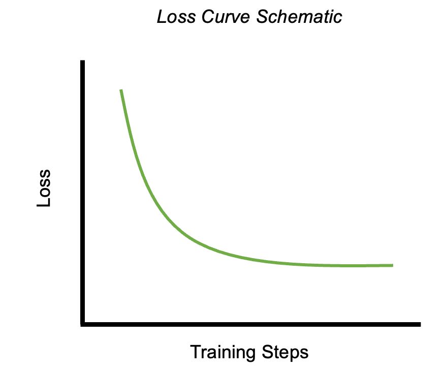
Each “point” in a loss curve typically reflects an average across many contexts. That is, an LLM at a given training step might be presented with thousands of examples, and the loss (surprisal) is calculated for each token in each example. That means changes in performance reflect changes in an LLM’s ability to predict tokens on average.

That’s obviously useful for benchmarking overall training progress. But an average, of course, bundles together many potentially disparate phenomena, which makes it difficult to determine what an LLM is learning, when. To oversimplify a bit: suppose that an LLM needs to learn things like part-of-speech, basic grammatical constructions, and which words have similar meanings. One possibility is that each of these things are learned simultaneously, but another possibility is that they are learned at different stages of training. If the latter scenario is true, we’d need to disaggregate the loss measure to tease these stages apart.

Ultimately, on some level, we’ll still be measuring changes in the probability that a model assigns to various strings. The key difference is which strings we’re measuring the probability of, or what we’re comparing those probabilities to.

LLMs and n-grams: training “phases”?

One of my favorite articles taking a developmental approach comes from my former labmate, Tyler Chang. In this 2024 TACL article, Tyler (and co-authors) asked whether the developmental trajectories of relatively small models (~124M parameters) exhibited legible patterns. Specifically, they measured the surprisal each model assigned to input strings at each checkpoint, then asked which factors drove changes in the surprisal assigned to various strings.

Perhaps the most striking result comes from comparing the behavior of each model throughout training to the behavior of simple n-gram models (with varying n). An n-gram model is a type of language model that predates the transformer (or other “neural” architectures), and is much simpler conceptually: in an n-gram model, the probability of a given word directly follows from the number of times that word has occurred in some exact context of length n - 1.

To make this concrete, let’s consider a bigram model, i.e., in which n = 2. Here, the probability of word n following word n - 1 is determined by calculating the number of times n has immediately followed n - 1 in a corpus, then dividing by the number of times word n - 1 (the context) occurred overall. For example, if the string is “that iguana”, a bigram model would determine p(“iguana” | “that”) by first counting the number of times “that iguana” occurred in a corpus, then dividing this by the number of times “that” occurred in the corpus. This tells us: of all the times we’ve observed some context, how frequently did we see this particular continuation?

A bigram model is not a very good model of language: in most cases, the probability of a word cannot be deduced solely from the word immediately preceding it. Researchers can systematically vary n (the size of the window) to account for more or less context: when n = 1, the model reduces to a unigram frequency model (i.e., the frequency of each word in isolation); as n increases, the model accounts for more and more context, which can improve prediction accuracy—though it also runs into overfitting issues, which are typically addressed using various smoothing techniques.

In general, even n-gram models with smoothing are not particularly good models of language, in part because of their lack of representational flexibility: a key benefit of transformers and other “neural” approaches is that they represent strings in a vector-space, reflecting generalizations across specific strings (e.g., part-of-speech, semantic class, etc.), which allows models to make approximate predictions for strings they haven’t observed before. But this is also why n-gram models offer a useful “anchor” for studying the training dynamics of a transformer. By comparing a transformer language model’s predictions to different n-gram models, we can understand the patterns of apparent generalization that transformer is undergoing.

Specifically, for each training checkpoint, Tyler calculated the correlation between a language model’s predictions and the predictions made by n-gram models of varying n. The pattern they found was pretty clear:

Consistent with previous work (Chang and Bergen, 2022b; Karpathy et al., 2016 for LSTMs), the models overfit to unigram (token frequency) predictions then bigram predictions early in pre-training. Extending this up to 5-grams, the models reach maximal similarity to a unigram model around step 1K, before peaking in similarity to 2, 3, 4, and 5-grams, in that order.

That is, the transformer models appeared to follow different “stages” of training, in which predictions gradually reflected sensitivity to longer and longer contexts.

One way to think about this is that early on in training, the simplest and most effective way to minimize loss is to predict tokens on the basis of their individual frequency. If you don’t really know anything about language, you’re best off assigning high probability to very frequent words like “the”, and low probability to infrequent words like “zoologist”. Throughout training, however, the model learns longer and longer chunks, corresponding roughly to n-gram models of various sizes—until, eventually, it forms generalizations that allow it to make even more flexible, context-sensitive predictions that can’t easily be captured by an n-gram model.

This progressive pattern has been attested in many different models of different sizes, trained on different corpora (see, e.g., a paper by another former labmate, Michaelov et al., 2026). It seems, then, to be a relatively robust principle underlying language model training dynamics. This is crucial: identifying generalizable principles is central to the scientific endeavor, and the notion that language models undergo various “phases” during training is an important start towards this identification process.¹

Beyond n-grams: phases and more

Of course, there are many ways one could measure potential “phases”. Beyond comparing a language model’s predictions to the predictions of an n-gram model, researchers can also compare predictions between various language models, or they can ask about changes in response to some particular stimulus contrast.

The first approach allows researchers to determine whether and when the behavior of different models converges or diverges. By also manipulating things like the initial parameters of a model, the data it’s trained on, or the model’s architecture, researchers can try to identify the model-level properties that drive patterns of convergence or divergence.

One recent paper (Fehlauer et al., 2025) adopted this approach using random “seeds” of the PolyPythia suite: these are open-source models trained on exactly the same data in the same order, but initialized with different parameters. Here, at each checkpoint of a given architecture, the authors compared the output probability distribution between random seeds, using a measure that captured the degree to which two probability distributions converge or diverge. Then they visualized these patterns of convergence across pretraining. As depicted below, they found evidence for roughly four distinct “phases”: first, a uniform phase (i.e., before models have learned much about language); second, a sharp convergence pattern (i.e., when different models start resembling each other in their predictions); third, a divergence pattern (i.e., models start looking rather different); and fourth, a slow reconvergence pattern (i.e., models of the same architecture again start to resemble each other).

Patterns of convergence and divergence between random seeds of the same model across training. Figure taken from Fehlauer et al. (2025).

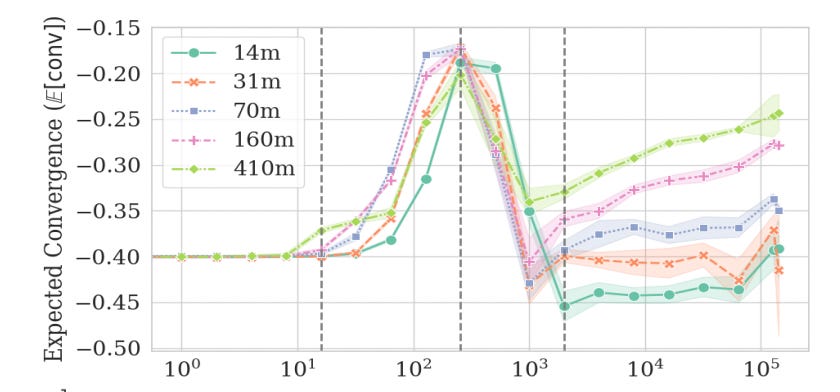
One of the most interesting things about this result, in my view, is the differences across model sizes. All models undergo the first three phases (i.e., uniform, sharp convergence, and divergence), but the smaller models exhibit less evidence of reconvergence, or seem to do so more slowly. What causes this gap? A speculative explanation lies in the factors causing convergence and divergence in the first place: given what we already know about correlations with various n-gram models, a reasonable hypothesis is that early convergence between transformer language models is driven by relatively simple n-gram statistics (e.g., unigram or bigram frequency), which even small models can learn. Divergence is then driven (perhaps) by subtly different patterns of generalization across models. Finally, the slow pattern of reconvergence—most pronounced in larger models—is, possibly, driven by those models all converging on the “same” generative account of language.

For what it’s worth, I’ve observed very similar patterns in my own work, examining a range of different model behaviors. That is, seeds of larger models exhibit more pairwise similarity than do seeds of smaller models, and they also converge earlier, and faster, than do seeds of smaller models. For example, here’s an analysis looking at inter-seed correlations in when and to what extent different Pythia random seeds learn particular dative constructions (e.g., “I gave him the ball” vs. “I gave the ball to him”). I won’t go into too much of the linguistic details here, but the quick version is that different ways of expressing a transfer event are preferred in different situations, according to what’s being described (e.g., “the ball” vs. “the curious object I found in the grass”) and the surrounding discourse context (e.g., what’s already been mentioned, etc.). In a recent project, I calculated the “preference” language models have for these different constructions at different checkpoints, then compared these preferences both across language models and to humans. The pattern of inter-seed converge and divergence is depicted below:

Inter-seed convergence and divergence in preferences for various dative constructions. Figure from work in progress.

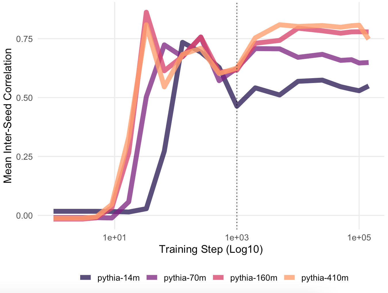
Early on, seeds exhibit little to no correlation with each other: they don’t know anything about the dative construction. After observing about 0.5B-1B tokens, seeds exhibit a sharp convergence pattern (though larger models do so earlier than smaller models). This is followed by a temporary “dip”, which is in turn followed (in larger models) by a reconvergence.

I’ve now analyzed the training dynamics of various behaviors and internal mechanisms, and I’ve found very similar patterns in each case. First, there are relatively clear “phases” of convergence and divergence between random seeds of the same model across training. And second, models show systematic variance in these patterns as a function of their size. Larger models tend to converge earlier, faster, and to a greater extent than smaller models.

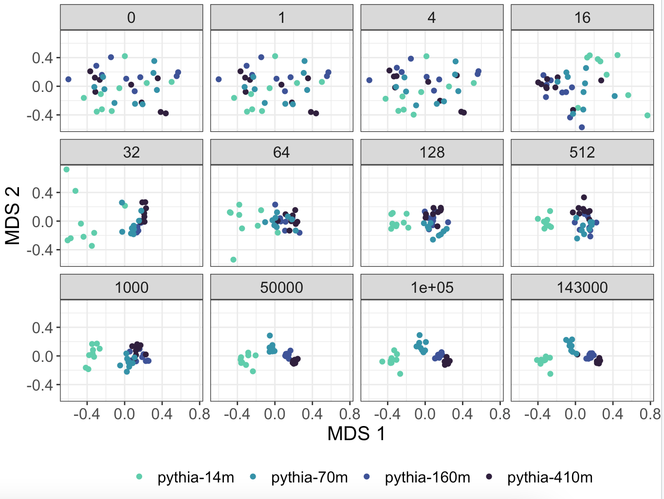
Another way to visualize this latter claim is to embed each seed of each model in a two-dimensional space using something called multi-dimensional scaling (MDS). To do this, I first calculated (at each checkpoint) the correlation in output predictions between every pair of models: this tells us the extent to which one model instance is “aligned” with another in terms of its predictions. This produces a correlation matrix of size MxM (where M is the total number of model instances). Then, for each checkpoint, I ran MDS on this correlation matrix, which projects it into a two-dimensional space preserving some of the original structure. These new dimensions aren’t intrinsically meaningful or interpretable, but they reflect the original similarity structure of the correlation matrix: that is, model instances with more similar patterns of correlations will be closer together in the 2D space. By running this process at various checkpoints, we can observe how different model instances are “distributed” throughout the 2D space, and how that process evolves throughout training.

The figure below depicts the MDS projection at different stages of training. Each point represents a particular seed of a particular model architecture, and the points are colored according to their size. As the figure depicts, points are roughly randomly distributed throughout the space early on in training, reflecting the fact that they haven’t really learned anything about language yet. As training progresses, however, model instances begin to converge. This is particularly true for seeds of larger models: e.g., in panels 32-64, we see that seeds of larger models cluster tightly together, while seeds of pythia-14m (the smallest model) are more sparsely distributed. Finally, in the latest stages of training, each model architecture exhibits relatively tight clustering, though notably, the cluster of pythia-14m seeds is somewhat distinct from the clusters of seeds for larger models.

Results of running multi-dimensional scaling on the correlation matrix of dative alternation preferences across pairs of language model seeds at each checkpoint. Figure taken from work in progress.

Behavior and mechanism, together

So far, I’ve discussed how particular behaviors change across training. But part of the promise of a developmental approach is that researchers can investigate changes not only in behavior, but in the internal mechanisms and representations of language models as well. Moreover, by analyzing how these changes coincide, researchers can get better conceptual traction on how exactly internal mechanisms give rise to observable behaviors. This kind of approach has been applied to a number of domains, including how and when models learn syntactic constructions, which mechanisms underlie in-context learning, and more.

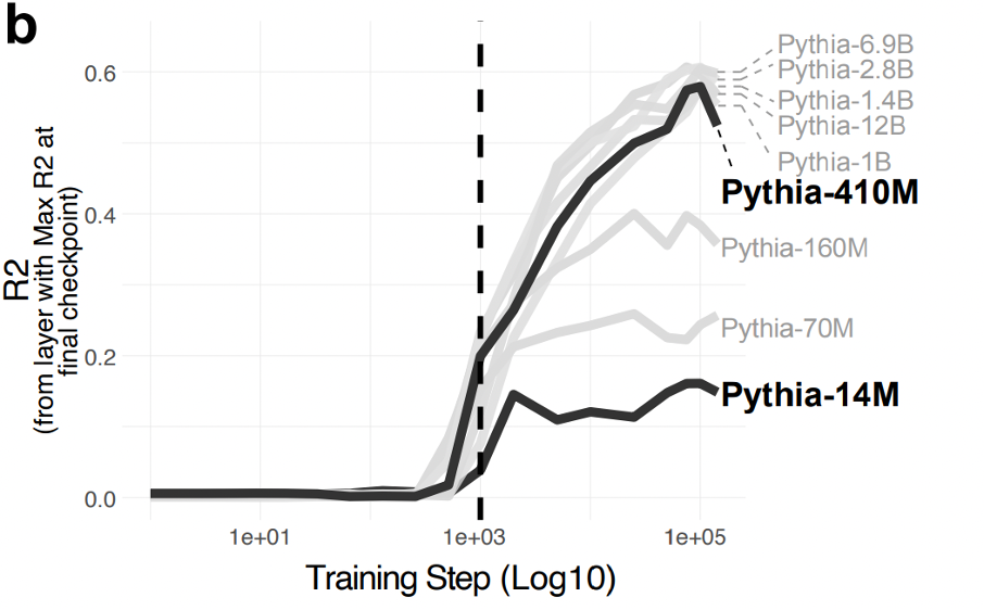
This is also the approach Pam and I adopted in a recent paper. We focused on the ability of language models to disambiguate the meaning of a word in context. Specifically, we asked whether and when language model representations of ambiguous words (e.g., “lamb”) reflected human similarity judgments. The sense of lamb evoked in “marinated lamb” is distinct from the sense evoked in “friendly lamb”, but is more similar to “roasted lamb”. As a proxy for disambiguation behavior across training, we compared the similarity of language model representations for words in different contexts to human relatedness judgments about these words. We found, first, a relatively sharp inflection point around step 1K (about ~2B tokens observed), at which point each model we tested started showing evidence of disambiguation. Again, larger models continued improving well past this point, while smaller models seemed to plateau:

Performance of various language models in the Pythia suite throughout pretraining. R2 reflects proportion of variance explained in human judgments using cosine distance from that language model’s best-performing layer. Figure taken from Rivière & Trott (2026).

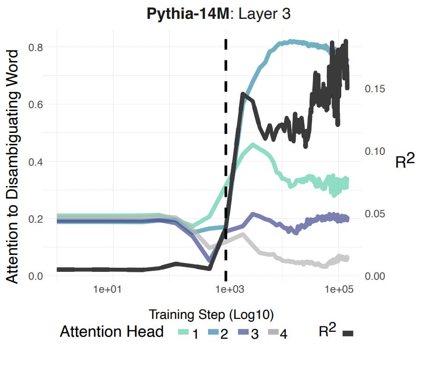
We then turned to the mechanisms subserving these changes. One hypothesis we had was that specific attention heads might learn to attend to specific cues that helped disambiguate a target ambiguous words. Fortunately, our stimuli were designed such that there was always a single disambiguating cue (e.g., “She liked the marinated lamb”). For each attention head in each model, we measured the attention strength from the target ambiguous word (e.g., “lamb”) to the disambiguating cue (e.g., “marinated”), and visualized these changes over training. Our goal was to find heads that attended strongly to the disambiguating cue—and, crucially, which exhibited a similar developmental trajectory as the overall disambiguation trajectory.

The figure below depicts the pattern of attention to disambiguating cues for the four attention heads in layer 3 of pythia-14m, superimposed over the model-level changes in disambiguation performance (measured as R^2). Here, I’ll make two observations. First, the heads in this layer are clearly not all doing the same thing. Two heads (3 and 4) don’t really “look” at the disambiguating cue at all, whereas the other two heads (1 and 2) do show a stronger pattern of attention to the disambiguating cue (especially head 2). And second, these changes in attention are timelocked to changes in disambiguation behavior!

Attention from a target ambiguous word (e.g., “lamb”) to disambiguating cue (e.g., “marinated”) from each head in layer 3 of pythia-14m, superimposed over model-level changes in disambiguation performance. Figure adapted from Rivière & Trott (2026).

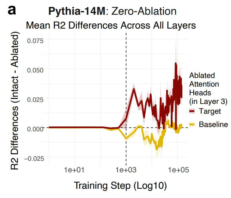
Of course, this doesn’t entail that these attention heads are therefore functionally involved in disambiguation. But it does suggest that there’s a temporal synchrony in when specific mechanisms begin reorganizing their behavior and when the overall model begins to improve in disambiguation. To test the functional role of these attention heads, we’d need to intervene on them (e.g., “knock them out”) and ask how this affects changes in behavior. Thus, we carried out a series of ablation studies in which we systematically altered the behavior of those attention heads and asked how much this “hurt” disambiguation performance, as compared to ablating random heads. We did this at each checkpoint of the model. As depicted below, we found that ablating the target heads did impair performance (compared to the baseline heads), and did so throughout training. Moreover, these ablations didn’t affect performance early on in training, which is exactly what you’d expect given that the model hasn’t learned the disambiguation behavior at this point yet.

Effects of ablating target heads at various checkpoints, as compared to ablating random baseline heads. Figure adapted from Rivière & Trott (2026).

A few caveats are in order. First, these ablations reduced performance, but they didn’t entirely knock it out. This was particularly true for larger models, in which there was considerable redundancy across attention heads: thus, it stands to reason that knocking out any individual head wouldn’t have a huge effect on performance.

Second, this doesn’t entail that these heads are therefore “disambiguation heads”. Indeed, determining the functional scope of a model component is in part a philosophical problem, which depends on carefully defining the conceptual boundaries of a behavior or mechanism. We carried out a range of “stress tests” to determine the robustness of each head’s behavior to various stimulus perturbations. These are described in more detail in the paper, but briefly: heads of smaller models were not particularly robust to these perturbations, suggesting that they perform relatively simple operations (e.g., “1-back heads”); in contrast, heads of larger models were less brittle, suggesting they might perform a more generalizable operation (e.g., “noun modification”) robust to the part-of-speech or relative position of the disambiguating cue.

Third, and perhaps most importantly, this is a relatively simple behavior, characterized in only a handful of models. As I’ve written before—and as others have argued as well—a fully developed science of LLMs will depend on identifying robust, generalizable behaviors and mechanisms across LLMs that enable us to make accurate predictions about those models.

Causal history as an epistemic criterion

I’ve spent much of the last year or so thinking about the key epistemological challenges facing LLM-ology. Those challenges include questions of generalizability (which findings generalize to which models?), construct validity (how do we know if we’re measuring what we think we are?), and ontology (what kind of thing is an LLM anyway, and how ought we study it?). During this period, I’ve been reading more history and philosophy of science, trying to contextualize these questions in the challenges other disciplines have faced. The position I’ve gradually arrived at is something like a coherentist approach to the study of LLMs: for the most part, I don’t think we’ll ever identify procedures for producing determinative answers or conclusions about LLMs—instead, I think researchers need to carefully articulate their explanatory goals and theoretical commitments, then contextualize their claims in a “justificatory web” of mutually supporting pieces of evidence, which will offer a provisional understanding of how these systems work in the service of particular theoretical or practical goals.

The reason I bring this up is that I think such a perspective necessitates consideration of what might constitute this “justificatory web”. As I’ve written before, I think the scientific study of LLMs should be rooted, in part, in an attempt to understand them “on their own terms”. I continue to believe the lens of Cognitive Science can provide a useful perspective—at minimum, deriving inspiration from careful experimental design and control—but I’m also quite open to the possibility that a theory of LLMs might well be grounded in something that looks very different from a science of human cognition.

What might that be? Well, one very important property of language models is that they are trained. This training process can be viewed as an effective procedure for producing a configuration of weights that produces the kinds of behaviors we find so interesting. If we’re to understand LLMs on their own terms, I think we need to think of their training dynamics as central to the kind of thing they are. This is akin to an argument made in Biderman et al. (2026), which describes models as time-evolving processes:

Answering the question “why did a model do X on Y input” certainly has some utility (e.g. for corporations interested in product assurance, user-satisfaction, and compliance), but on a scientific level it’s fundamentally limited. A more scientific mindset would be to ask “why did the model develop this behavior?” This involves shifting from viewing models as static objects to viewing them as snapshots of time-evolving processes and studying the entire dynamical system (Saphra, 2023; Biderman et al., 2023b; Hoogland et al., 2023). When the object of study is the training process rather than the finished model, an account of that process can be applied [to] any model it produces, not to one specific set of weights (Sellam et al., 2022). (pg. 3)

There are still, of course, considerable degrees of freedom in how behaviors are characterized, and in the kinds of explanations for this behavior we might investigate or find satisfying. I’d advocate for pluralism in this respect: I think the field is too nascent to warrant extreme confidence about the right level of analysis here. But I do think that a scientific understanding of LLMs should be informed by an understanding of their causal histories, i.e., the story of how they got their weights.

1. Note that when researchers in this space use words like “phase” or “phase transition”, they’re usually referring to something like a sharp discontinuity in some measurable behavior over the course of training, as opposed to incremental changes. The question of whether these behaviors should be called “emergent” has received some attention, given that “emergent” has specific meanings in the study of complex systems. For the purposes of this post, I’ll be using words like “phase shifts” in the sense described above—i.e., as sudden changes in some target behavior over the course of training.