
A couple months ago, readers voted on some topics they’d like to see me cover; one of them was an explainer on techniques for model distillation and building more efficient LLMs generally.
State-of-the-art large language models (LLMs) require huge amounts of resources to train and deploy. Historically, most of this cost has come from training (training GPT-4 is estimated to have cost about $100M), though widespread usage has also increased the total costs associated with deployment, especially with the rise of chain-of-thought “reasoning” techniques.
Naturally, there’s considerable interest in reducing these costs. The companies building these models would presumably like to spend less money on compute, assuming they could guarantee similar performance. Moreover, these processes are expensive because they use lots of energy, much of which involves some amount of carbon emissions1: while there’s reasonable debates about how to quantify and assess the actual environmental harms, it seems (to me, at least) straightforwardly true that training and deploying models more efficiently would reduce whatever environmental harms there are.2
Finally, there are more theoretical reasons to prefer more efficient models—particularly if by “more efficient” we mean smaller and/or trained on less data. As I’ve written before, humans seem to acquire remarkable linguistic competence despite encountering fewer words than LLMs; theories of language learning would be informed by the success or failures associated with training models on more plausible volumes of linguistic input. Similarly, smaller models may be more interpretable than larger ones: intuitively, it seems easier to try to understand 100M parameters than 100B parameters (though whether or not this is actually true remains to be seen3). And from a purely self-interested perspective, I think basic scientific research on LLMs would benefit from more efficient models: it’s hard to run (and even harder to train) state-of-the-art LLMs on an academic budget, which limits the kinds of questions we can ask.
With all that in mind: why is it that models are so expensive to train and deploy, and what are researchers doing to reduce these costs?
Why are models so hungry for compute?
We can roughly divide compute costs into those associated with training and those associated with inference.
Before training, an LLM consists of layer upon layer of random weights (or “parameters”). Such an LLM could be used to generate predictions about upcoming words, but those predictions would be very bad: we might say (informally) that it doesn’t “know” anything about language. Typically, training consists of presenting many examples from a language corpus to the model and comparing its predictions to the actual word in a given context. Learning, then, is informed by an error signal. The model’s mistakes are used to make “updates” to the parameters; over time, these updates produce parameters that make better predictions.
The reason I’m describing these details—and there’s lots I’m glossing over—is that an intuition for what training involves is helpful for understanding why it’s so compute-hungry. Concretely, an “update” to the model looks like something like this:
Pass in a sentence or “batch” of sentences and run a “forward pass” through the model (i.e., derive predictions for each example).
Compute the error associated with each prediction.
Use that error to figure out how to update each model parameter; the technique for “walking” the error backwards through each layer is called backpropagation.
Each of these steps must be performed for each training example, and datasets often contain billions or trillions of tokens. Moreover, in a state-of-the-art LLM, there are often tens of billions or even hundreds of billions of parameters4, each of which must be used in calculations during each forward pass and subsequently updated based on the error signal from each training example. To make matters worse, successful training often involves multiple passes through the dataset, meaning each example might be observed many times by the model. Finally, because of how attention in transformer LLMs works (more on that below), longer and longer context windows produce quadratic increases in compute costs.
That’s a lot of calculations! As we wrote in our explainer on LLMs:
OpenAI estimates that it took more than 300 billion trillion floating point calculations to train GPT-3—that’s months of work for dozens of high-end computer chips.
Another way to get intuition for this is to think about what it would take to do all this by hand. As I’ve written before, even a single forward pass through the model could take thousands of years.5 That’s not even considering the calculations involved in computing the error signal and backpropagating that signal through the network to update the weights.
That’s training. Inference refers to using the model purely for a forward pass—that is, with the “weights frozen” so that no updates are made based on the model’s output. This should already give you some intuition as to why inference is generally cheaper than training: training a model requires both a forward and backward pass through the model. That said, as Tim Lee has written, inference costs are now non-trivial. We can attribute that to a few causes: first, more people are using tools like ChatGPT, and each “query” involves a number of forward passes involved in generating the model’s response tokens; second, models and context windows have gotten bigger and bigger; and third, models increasingly deploy chain-of-thought or “scratchpad” techniques, which involve generating lots of tokens on the “path” to producing the final answer.6
Understanding this context is (hopefully) useful for understanding how researchers might in turn make headway on building more efficient models. A few techniques are focused on training models more efficiently, while others are focused on deploying an already-trained more efficiently. The rest of this post will walk through some of the techniques researchers are exploring. Because there are more techniques aimed at making already-trained models more efficient, that’ll be the primary focus—but I’ll also discuss some of the efforts to speed up training towards the end.
Knowledge distillation
Knowledge distillation (KD) refers to the process of compressing (or “distilling”) the representations and functions (or “knowledge”) of a large model into a smaller model. You can think of KD as a general class or approach, as there are many specific techniques for implementing it. The goal of knowledge distillation is to a produce a smaller, more efficient model from a bigger, already-trained model: thus, it’s a technique for making deployment more efficient.
The core intuition is that a large model is able to extract complex relationships from its training data that a small model might not be able to. Once trained, however, it may be possible to use the representations or outputs from that large model as a training signal for a smaller model. That is, the large model may produce representations that serve as a helpful training signal for a smaller model—perhaps more helpful than the original training data.
There are various reasons why this might be true, but one way of thinking about this is that the original training signal is sometimes pretty coarse. Consider an image classifier trained to sort images into the following bins: cats, dogs, tables, and other. Typically, that classifier will be trained on images with a single label (e.g., “cat”), and its error signal will thus fail to incorporate the similarities between the classes of interest. Suppose, for instance, that the model misclassifies a picture of a cat as a dog; intuitively, this seems like a less egregious error than misclassifying it as a table, but a typical training signal will simply take into account the probability assigned to cat.
The direct training signal for LLMs is similarly coarse. Typically, an LLM is penalized according to (essentially) the inverse probability7 assigned to the correct token in a given context: specifically, assigning a probability of 1 (100%) to the correct word would result in a loss of 0, resulting in no penalty; anything less than a probability of 1 results in a larger loss (thus necessitating updates to the weights). But clearly, some mistakes are larger than others, and it seems plausible that predicting the word “car” when the correct word is “automobile” should incur a smaller cost than predicting “elephant”.
In both cases, the challenge arises from the fact that learning to classify hard labels (a given token or image category) doesn’t take into account that there is useful information in the kinds of errors a model makes; Geoff Hinton once called this “dark knowledge”. Of course, it’s not that engineers are unaware of this fact! It’s just much harder to identify a scalable metric for penalizing models in this way—and large-enough models seem to achieve pretty good performance with the training protocols we already use, even if smaller models struggle to get off the ground.
To return to where we started: model size may be a useful proxy for a model’s capacity to extract complex relationships from the training data even with a somewhat coarse error signal. Concretely, a larger model contains more possible “sub-models” (Frankle & Carbin, 2018) and thus more opportunities to identify the function that best approximates the data.8 The insight of knowledge distillation is that once that large model has been trained, we may not need all those parameters to perform the same computations. Instead, we can distill the hard-won knowledge from the bigger model into a smaller model by exploiting the observation above: there is information is the kinds of errors or representations produced by that bigger model, which acts as finer-grained training signal for a smaller model.
One specific technique is known as logit distillation (Gou et al., 2021). The idea here is that we can the outputs of a bigger “teacher” model—the probabilities assigned to each possible token or image label—as a training signal for a smaller “student” model. The procedure looks something like this:
Researchers present the same input (e.g., a sentence or image) to the already-trained teacher model and untrained student model.
They then extract the outputs (e.g., logits or probability distribution) from the teacher model.
Those outputs are used as the training signal for the student model (i.e., instead of simply measuring the probability assigned to the correct output).
This procedure is depicted in the visual illustration below.
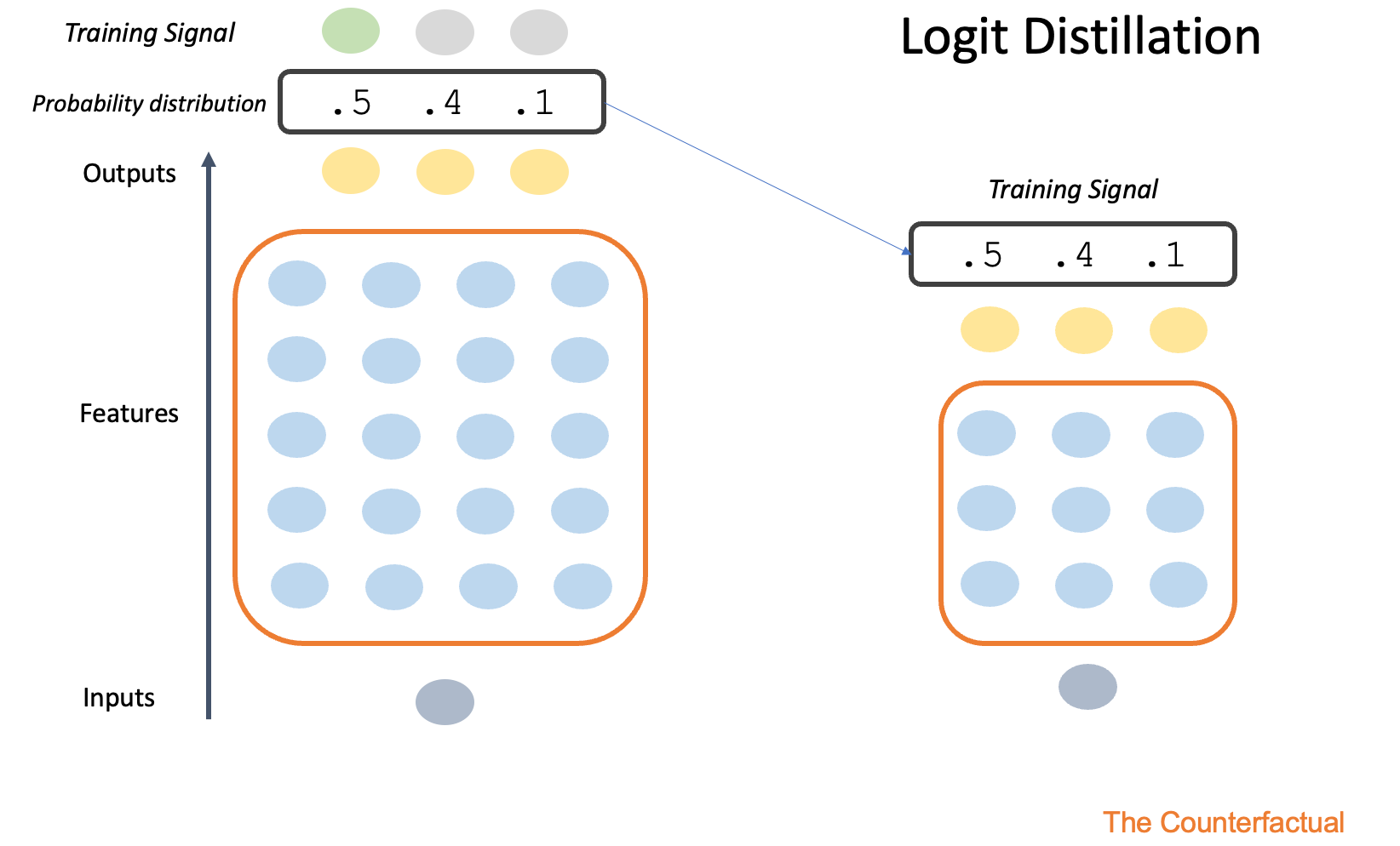
Empirically, techniques like logit distillation can work surprisingly well. The benefit, of course, is that the end result is a smaller model that runs more efficiently and, at least in principle, is about as good as the bigger model. A related approach is to train the smaller model on the features (i.e., internal representations) from the bigger model, as opposed to the outputs; this approach is sometimes called feature distillation.
More recently, researchers have explored other techniques, enabled by the success of systems like LLMs in generating content (like coherent paragraphs). One such technique (discussed in this survey; Yang et al., 2024) is called In-Context Learning Distillation. In-context learning (ICL) consists of presenting an LLM with a series of questions and answers (or example tasks) in the “context” of the question or task the user wants the LLM to solve; the examples in the context help steer the LLM towards the kinds of responses the user is looking for.9 You can think of ICL Distillation, then, as a kind of modified version of logit distillation, using generated sequences as the training signal instead of the logits. A teacher model (say, GPT-4) is presented with a given context and asked to generate some output; that entire string (context + output) is then presented to a student as the training signal to mimic.
The advent of “reasoning” approaches like chain-of-thought (CoT) have also motivated researchers to train on these generated sequences as well. Here, the approach is similar to ICL Distillation, but the teacher model is asked to produce a series of reasoning “steps” involved in producing a given answer; the student model can then be trained directly on those steps. If we assume that the reasoning steps in the teacher model are correct—a nontrivial assumption, to be clear—this has the advantage of automatically producing a training signal for elaborate reasoning chains.
These latter techniques are sometimes called “black-box distillation techniques” because the student model is not being trained directly with representations or logits from the teacher—instead, the generated behavior (token sequences) of the teacher model is used as the target of training. Nonetheless, the approaches are conceptually analogous to some extent: in each case, a student model is trained to reproduce the outputs (logit distillation or ICL Distillation) and/or intermediate steps (feature distillation and CoT distillation) of a teacher model.
Why does any of this work? We can’t know for sure, but I think part of the answer comes back to what I mentioned earlier: bigger models might be better than small models at extracting useful information from a coarse training signal—but once that information has been extracted, it’s possible to distill it into a more compressed form. Of course, it’s also hard to judge how reliable the approach is: even if the smaller model performs equally well on certain benchmarks as the larger models, it’s always possible that we’ve “distilled away” truly important representations or mechanisms—we just can’t detect it in the benchmarks because measuring model capabilities is really hard. I’ll discuss this challenge more later in the post, but one possibility is that mechanistic interpretability techniques could help us decompose the teacher and student model to determine whether they are, in fact, performing similar functions, or whether the student is implementing more “superficial” heuristics.
Pruning
Like knowledge distillation, pruning assumes that once a large model has been trained, there exists some smaller model that can perform roughly the same set of functions about as well as the larger model. Pruning is thus also similar to distillation in that it boosts efficiency during inference, not training.
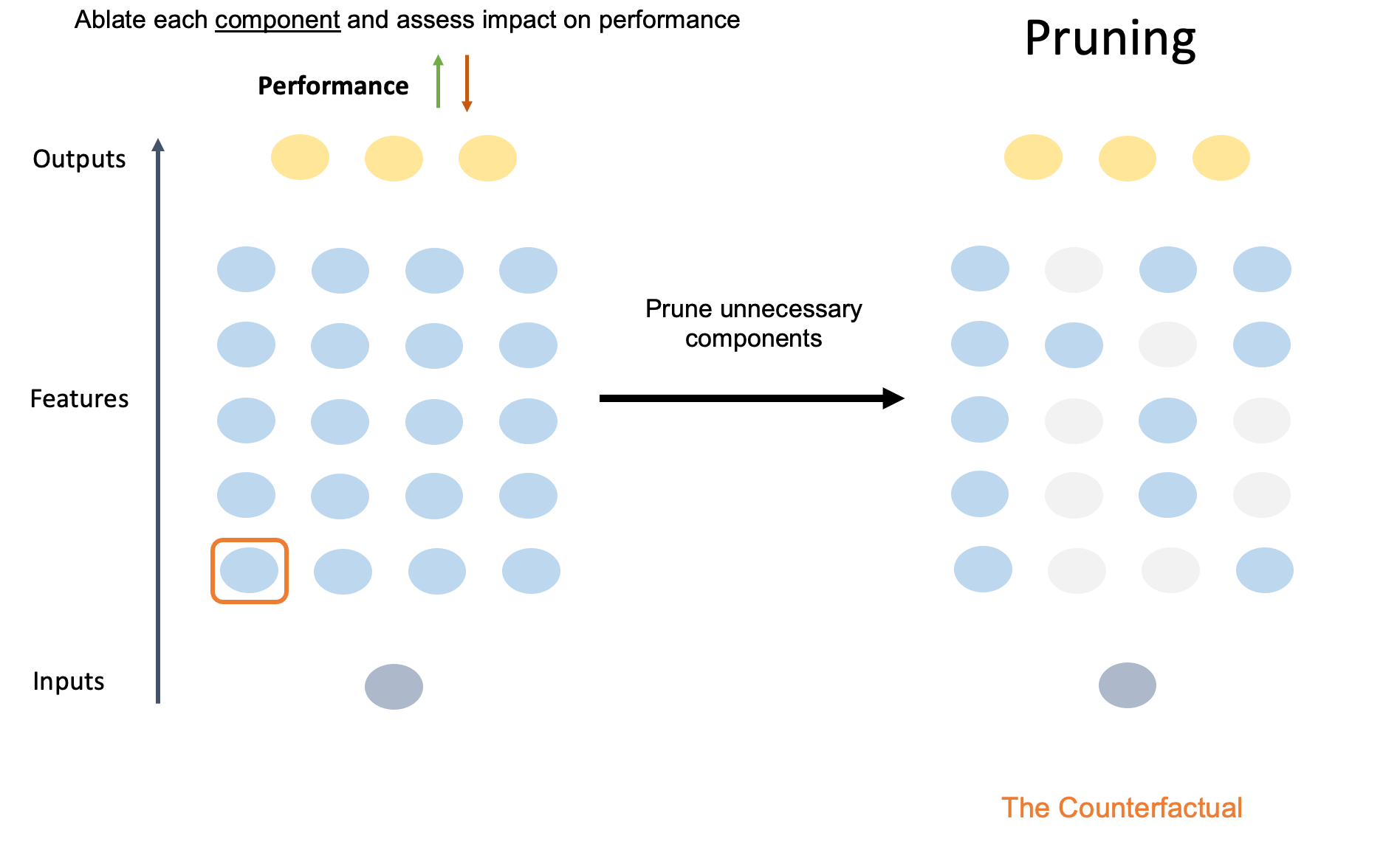
Unlike knowledge distillation, however, pruning works by systematically removing (or “pruning”) components of the original model directly. The resulting model is thus sparser: many of the original parameters have been set to 0.
The underlying assumption of pruning is that many of the parameters in the original model are somehow redundant or not particularly important. That is, the original model is overparameterized. Indeed, evidence for apparent redundancy—at least for select tasks—in transformer language models dates back at least to a 2019 paper (Michel et al., 2019) entitled “Are 16 Heads Really Better Than One?” The paper’s central question is right there in the title: most transformer models use multi-headed attention, meaning that each layer of the model has multiple “heads”, each of which could (in theory) learn to track different kinds of relationships in the context—but are all these heads really necessary?
The authors tested this question using an ablation study, a technique I’ve written about before. Ablation involves removing or “knocking out” different components of a model and asking whether the model’s performance on some task changes at all. The logic is that if a component is important for solving a task, then performance should decrease when that component has been ablated; if the component is redundant or unnecessary, then performance should not change. Concretely, the difference in performance between the original model and the version with a given component ablated is a measure of how much that component mattered for the task.
The authors focused on two models: WMT, the original transformer architecture from the famous “Attention is all you need” paper (Vaswani et al., 2017), which has 6 layers and 16 heads per layer; and BERT, which was considered “state of the art” at the time (though no longer), and which has 12 layers with 12 attention heads each. For each model, the authors applied the same procedure: one by one, they selectively ablated each head in each layer and quantified the resulting change in performance on a machine translation task. This amounts to asking how much worse WMT and BERT performed when equipped with one fewer head than the model was originally trained with. The authors found that removing most heads didn’t matter much (bolding mine):
Notably, we see that only 8 (out of 96) heads cause a statistically significant change in performance when they are removed from the model, half of which actually result in a higher BLEU score. This leads us to our first observation: at test time, most heads are redundant given the rest of the model.
But removing one of 96 (or 144) heads isn’t actually ablating a huge chunk of the model. In the next experiment, the authors inverted the approach from the first study: instead of ablating only a single head, they ablated all heads but one from a given layer, allowing them to ask whether that head was sufficient for solving a given task. Strikingly, they found that for some layers, one head was enough to retain good performance on the machine translation task:
We find that, for most layers, one head is indeed sufficient at test time, even though the network was trained with 12 or 16 attention heads.
The authors also report the difference in runtime efficiency between the original model and the pruned versions: unsurprisingly, pruning resulted in substantive efficiency gains.
Of course, as the authors note, these results were obtained for a specific task (machine translation) on specific models. It’s unclear how well they’d generalize to other tasks or other models, and there’s always a risk of being too eager to attribute redundancy to a system: maybe those other heads were important but it’s just hard to measure them. But I think the paper is primarily interesting as a proof-of-concept, both in terms of the method used (pruning) and the results (for a machine translation task, one head is sometimes as good as 12 or 16).
There is a growing body of work exploring redundancy in pre-trained transformer models, particularly with respect to the attention heads. Again focusing on machine translation, this 2019 paper (Voita et al., 2019) trained multiple transformer models to perform the translation task. They then ranked the relative “importance” of each head (the extent to which it impacted the model’s predictions), as well as its “confidence” (the average maximum attention to particular tokens10): in general, a small number of heads emerged as most “important”, and importance was positively correlated with head confidence. That is, heads that consistently distributed attention to particular tokens (as opposed to distributing it more uniformly across tokens) made stronger contributions to model outputs.
The authors then characterized the putative function of the most important heads by analyzing their attention matrices, classifying them as follows:
Positional heads were those that consistently (≥90% of the time) attended to specific relative token positions (e.g., 1-back heads).
Syntactic heads were those whose attention weights correlated with particular syntactic dependencies, e.g., subject-verb relations.
Rare word heads tended to point towards the least frequent token in a sequence.
One of the things I found most interesting about this paper was that these “important” heads really did seem to have relatively interpretable functions. Moreover, these functions actually make sense in the context of what the models were trained to do: at minimum, translating from one language to another seems like it would benefit from paying attention to the relative position of words in the input and output sequence, the syntactic relations of those words, and the use of particularly unusual or infrequent words. (This is a good place to note that a good machine translation model would almost certainly need to pay attention to more than just those things; it’s also entirely possible that the heads analyzed performed more complex or sophisticated functions that were simply harder to characterize.11)
But again: these are small models trained on a specific task, and we should be cautious about extrapolating to other model classes or task contexts.
Setting aside, for now, the question of whether and which model components might be redundant, we can turn to a second, equally challenging question: given that our goal is to identify some subset of a model’s parameters that are sufficient for equivalent performance, what’s the best way to identify that subset? This is a version of what’s called model selection in statistics and machine learning.
Naively, one might imagine that you could find the “best” model simply by testing every possible subset of parameters. But this quickly becomes computationally intractable. Suppose you have 100 parameters (k = 100), and are willing to entertain subset models ranging from those with no parameters (k = 0) to those dropping only a single parameter (k = 99)—and everything in between. There are roughly 10^30 such possible models. If we assume each candidate model takes only one second to fit and evaluate, it would take 10^30 seconds to evaluate all those candidates: for comparison, the likely age of the universe is about 10^17 seconds. That means it would take longer than the entire history of the universe thus far simply to identify the best subset of 100 possible parameters for a given task.
Clearly, we need a better way. There are a number of different model selection techniques used in statistics, such as forward or backward stepwise regression, in which variables are added or removed one at a time according to some evaluation criterion; researchers also make use of regularization methods like Lasso, which impose an additional sparsity constraint on the final model. These methods don’t necessarily find the globally optimal set of parameters, but they work well as heuristics for finding a “good enough” model.
Similar principles apply in the context of pruning neural networks, though the scale and complexity of the problem is considerably greater than most linear regressions. “Greedy search” methods make the best locally optimal choice at each decision point and are roughly analogous to stepwise regression. For instance, you might start by finding the best single attention head out of all possible attention heads (say, 100)12; once you’ve found that head, you proceed by finding the best second head to add to that head out of the remaining heads (99); you then continue this process until you’ve added all heads in order of importance.13 This might still take a while—especially if you have many attention heads—but it’s much, much faster than searching all possible combinations of heads.
In general, pruning methods tend to trade off between computational complexity (i.e., the efficiency of the pruning procedure) and fidelity (i.e., whether you end up removing the right parameters). These range from removing parameters with the smallest magnitudes (highly efficient, but imprecise) to more sophisticated methods like the “Optimal Brain Surgeon” and its modern counterparts. The most accurate methods tend to rely on “second-order” metrics that account for the curvature of the overall loss landscape when removing model parameters; this is in contrast to “first-order” metrics that use only the local gradient information (i.e., increases or decreases in loss) to estimate a parameter’s impact. (Metrics like parameter magnitude could be considered “zeroth-order” in the sense that they’re not calculated as a function of the loss at all.) Unfortunately, second-order metrics are the most expensive to compute, whereas zeroth-order metrics are much faster. There are, however, clever workarounds that attempt to balance these trade-offs. For instance, the SparseGPT method relies on second-order metrics, but computes them layer by layer (as opposed to the entire model) using relatively efficient methods, which makes the problem more computationally tractable.
Putting this all in context: like knowledge distillation, the key assumption of pruning is that many LLMs are overparameterized—they have more parameters than they need. In principle, then, one could identify a subset of these parameters that runs more efficiently without a loss in performance. The main challenge is figuring out which parameters are actually necessary and which are redundant, and doing this in a way that doesn’t take longer than the age of the universe to calculate.
What about training?
So far, I’ve focused on methods that make already-trained models run more efficiently. But as I wrote earlier, much of the energy costs come from training. Can we speed that up as well?
Training has indeed gotten more efficient in some ways, mostly through a combination of hardware advances and algorithmic approaches that better exploit these advances. Some benefits have come through improved optimization methods: while neural networks were historically trained using stochastic gradient descent (SGD), optimizers like Adam generally result in faster convergence than SGD by adapting the learning rates (how quickly parameters are updated) for each parameter based on its historical trajectory. Other techniques, such as mixed-precision training, reduce the precision of each stored weight (e.g., storing up to 8, rather than 16, decimal values), which speeds up both inference and training.
One innovative technique that’s been particularly impactful for making fine-tuning more efficient in particular is LoRA, or “low-rank adaptation” for LLMs (Hu et al., 2021). The underlying assumption of LoRA is that most of the changes to weight matrices induced by fine-tuning can actually be represented in a lower-dimensionality matrix than the original model matrices. That is, if the original matrix has 100 columns, you might be able to represent the changes to that matrix in terms of just 5-10 columns of updates.
Conceptually, this makes sense if we assume that fine-tuning mostly introduces a few new “directions” in weight-space, while keeping other aspects of weight-space relatively intact. Oversimplifying a bit: training on medical textbooks might introduce new information about medicine and health, but not necessarily new grammatical rules or general facts about the world. Thus, we might be able to represent those updates using fewer dimensions than the original weight matrix.
The technical details of LoRA are, of course, more complicated. LoRA works by “freezing” the actual weight matrix W (i.e., preventing it from updating) and instead learning updates to two smaller matrices: let’s call them A and B. Respectively, these matrices help summarize the core dimensions for the updates (A) and spread their influence (B) across all the original dimensions of W. Concretely, if W is 100x100 dimensions, A might be 100x10 and B might be 10x100. In this case, LoRA allows the model to learn roughly 10 “directions” of weight updates, which in turn can be distributed back across the original 100 dimensions. Thus, instead of learning updates for the full 100x100 grid (10K parameters total), LoRA would learn updates for each 10x100 grid (for a total of 2K parameters): a 5x reduction in the number of parameters the model had to learn!
In practice, the savings of LoRA are often even more dramatic. The authors of the original paper report as much as a 10,000x reduction (bolding mine) with no apparent loss in performance:
Compared to GPT-3 175B fine-tuned with Adam, LoRA can reduce the number of trainable parameters by 10,000 times and the GPU memory requirement by 3 times.
It’s worth noting that the logic here is, in some ways, similar to the ideas underlying knowledge distillation and pruning—only applied to the dimensionality of weight updates as opposed to the weights themselves. LoRA’s assumption is that when it comes to fine-tuning, updating every parameter in the full model would in some sense be an “overparameterized” update. Instead, this update can be distilled in a lower-rank matrix that nonetheless effectively summarizes the important directions of change.
LoRA has had a major impact on the field in terms of making fine-tuning much more efficient. Some researchers have tried to develop LoRA-like methods for pretraining as well, which have had some success, though my understanding is that their impact is considerably limited relative to LoRA. Again, this makes some conceptual sense if we keep in mind the distinction between training from scratch vs. fine-tuning: when training from scratch, the model “knows nothing” and thus likely benefits more from exploiting the full dimensionality of its parameters—if you could summarize the updates with fewer dimensions, you might just be able to use a smaller model in the first place. In fine-tuning, the model has already learned a lot about how language works, so the updates can be more targeted.
The age of small language models?
While I was writing this explainer, The Economist published an article suggesting that “small language models” (SLMs) might become increasingly relevant in the future. Aside from the fact that there’s something funny about calling them “SLMs”—the term large language model was coined to indicate a contrast with traditionally-sized (smaller) models of the past—I agree that smaller models are likely better-suited for many applications, especially any application that requires the model to run locally on a device.
And as I noted in the introduction, I also think there’s something philosophically interesting about trying to build more efficient systems. For the past several years, AI discourse has largely centered around the question of whether building bigger neural networks trained on more data will continue to yield performance improvements—sometimes called the scaling hypothesis. I think there’s merit to either side here, and I also think the debate about the exact shape of the function relating model size to model performance is interesting.14
But even if scaling holds to some degree, I like the idea of building systems that deploy resources more efficiently: not just because it’s financially or environmentally prudent (though this obviously matters too), but because much of what I find interesting about human cognition is the fact that it operates in a resource-constrained setting. Biological organisms operate under some pretty serious metabolic constraints; moreover, while the human brain is certainly energy-hungry, it’s seen by many as a remarkably efficient system in terms of what it achieves relative to its energetic costs. Efforts to do more with less might thus bring us closer towards building biologically plausible models of cognition.
The extent to which this is true is of course, is dependent on the grid used to power the data centers used to train the models.
At the very least, the ratio of harm to usage would decrease.
It’s possible that model with fewer parameters may end up “loading” more concepts into a smaller number of dimensions, which makes those dimensions hard to interpret. Techniques like sparse auto-encoders (SAEs) actually “explode” the dimensionality of a model, suggesting that in some cases, interpretability may be easier with more dimensions (though there’s ongoing debate about the utility of SAEs themselves).
We don’t know exactly how many parameters are in GPT-4, but some estimates are as high as 1.7 trillion. GPT-5 is a “multi-model system”, so each model in that system would have an associated number of parameters; even if we knew the parameter count of each constituent model, it’s not clear to me the best way to estimate the actual “parameter count” of GPT-5 itself.
The full post contains the assumptions needed to get this estimate, which include: the number of operations a person could perform per minute and the number of operations you’d need to perform. Obviously this is all back-of-the-napkin math, but my sense is that the order of magnitude seems roughly right. As I mentioned in the original post, if anyone disagrees with that estimate, let me know and I can correct it.
This is, in part, why leaderboards for benchmarks like ARC-AGI sometimes display performance relative to the compute costs required to solve a given task.
Or technically, the surprisal.
As described in that linked article, this is sometimes called the “lottery ticket hypothesis”. From the abstract:
Based on these results, we articulate the lottery ticket hypothesis: dense, randomly-initialized, feed-forward networks contain subnetworks (winning tickets) that—when trained in isolation— reach test accuracy comparable to the original network in a similar number of iterations. The winning tickets we find have won the initialization lottery: their connections have initial weights that make training particularly effective.
Technically, no “learning” occurs through weight updates—which is one reason for the popularity of the technique.
The logic here was that more “confident” heads tended to focus their attention on particular tokens, rather than distributing it across multiple tokens.
Another 2019 paper (Kovaleva et al., 2019) conducted an even more comprehensive analysis of putative head functions and attention patterns in BERT.
You could also do this in reverse, e.g., by starting with 100 heads and iteratively removing the heads that matter the least.
As described above, this won’t necessarily yield the optimal configuration of k heads, because the solution is path-dependent. It’s possible the best 6 heads are different than the best 5 heads plus the head that’s best to add next.
A fact that’s sometimes glossed over in contemporary discussion of the scaling hypothesis is that the original scaling laws paper actually showed some evidence of diminishing returns to model size. That doesn’t mean necessarily scaling has diminishing returns practically, just that the function relating performance to model size increases at a sub-linear rate. Of course, diminishing returns are still returns!
Great post! I always appreciate your dedication to citing notable and relevant papers - I always have so much interesting reading material at the end of each one of your blogs.
So well explained, Sean. Your students are very lucky!